MANGO LEAF DISEASE PREDICTION

In this assignment, we are given a dataset of images of mango leaves containing various diseases. There are 8 different diseases. Our goal is to classify an image into one of these diseases.

Convolutional neural network (CNN): CNN is an artificial neural network (ANN) which is mostly used in image classification. There are some disadvantages of using ANN for image classification. They are it involves too much computation, treats local pixels same as pixels far apart and sensitive to location of an object in an image. To overcome these problems, we use CNN. CNN uses filters to detect features in images. Filters are rotated throughout the whole image to detect features. After applying the filters over the image, we get feature maps. This whole process is convolution layer. We will use Relu activation function to the obtained feature maps. Relu helps with making model non-linear. Next pooling layer is applied to reduce the size to reduce computations. There could be any number of convolution and pooling layers. After that we will connect these to fully connected dense layer. CNN does not take care of rotation and scale. We have to use data augmentation techniques to generate new rotated, scaled images from existing dataset. As hyperparameters we have to specify how many filters to be used and size of each filter. 

Data Set Description: There are 8 directories. They are 'Anthracnose', 'Bacterial Canker', 'Cutting Weevil', 'Die Back', 'Gall Midge', 'Healthy', 'Powdery Mildew', 'Sooty Mould'. Each directory represents each disease.
 Inside each directory there are several leaf images. There are 4000 images in total.
 
Code:
 
1. In the first step I stored all the images present in the various directories in a data frame consisting of two columns img_path and class_names. In the first column there is path of the image and in the second column 
there will be corresponding disease name. 
 

data_dir = 'D:/Data/LeafData'

df = {"img_path":[],"class_names":[]}

for class_names in os.listdir(data_dir):

for img_path in glob.glob(f"{data_dir}/{class_names}/*":

df["img_path"].append(img_path)

df["class_names"].append(class_names)

df = pd.DataFrame(df)

2. The next step is to divide the data set into train, test, and development. I decided to split into 60% train, 20% test and 20% development.

from sklearn.model_selection import train_test_split

train_size=0.6

train,rem = train_test_split(df, train_size=0.6)

test_size = 0.5

dev,test = train_test_split(rem, test_size=0.5)

print(train.count())

print(dev.count())

print(test.count())

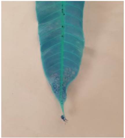
3. Next, I visualized one image

from PIL import Image

import numpy as np

from IPython.display import display

# define the shape of the image

height = 100

width = 100

channels = 3

pixel_values = cv2.imread(df.img_path[0])

image = Image.fromarray(pixel_values.astype('uint8'))

display(image)

Output:

4. Now, I used Label encoding to the class names.

from sklearn.preprocessing import LabelEncoder

Le = LabelEncoder()

train["class_names"] = Le.fit_transform(train["class_names"])

test["class_names"] = Le.fit_transform(test["class_names"])

dev["class_names"] = Le.fit_transform(dev["class_names"])

5. Next, I used One hot encoding to the class names.

train_labels=tf.keras.utils.to_categorical(train["class_names"])

dev_labels = tf.keras.utils.to_categorical(dev["class_names"])

test_labels = tf.keras.utils.to_categorical(test["class_names"])

6. In the next step, I performed image transformation and data augmentation.

def load(image , label):

image = tf.io.read_file(image)

image = tf.io.decode_jpeg(image , channels = 3)

return image , label

IMG_SIZE = 96

BATCH_SIZE = 64

resize = tf.keras.Sequential([

tf.keras.layers.experimental.preprocessing.Resizing(IMG_SIZE, IMG_SIZE)

])

data_augmentation = tf.keras.Sequential([

tf.keras.layers.experimental.preprocessing.RandomFlip("horizontal"),

tf.keras.layers.experimental.preprocessing.RandomRotation(0.1),

tf.keras.layers.experimental.preprocessing.RandomZoom(height_factor = (-0.1, -0.05))

])

7. Now I have written a function to create a TensorFlow data object .

AUTOTUNE = tf.data.experimental.AUTOTUNE #to find a good allocation of its CPU budget across all parameters

def get_dataset(paths , labels , train = True):

image_paths = tf.convert_to_tensor(paths)

labels = tf.convert_to_tensor(labels)

image_dataset = tf.data.Dataset.from_tensor_slices(image_paths)

label_dataset = tf.data.Dataset.from_tensor_slices(labels)

dataset = tf.data.Dataset.zip((image_dataset , label_dataset))

dataset = dataset.map(lambda image , label : load(image , label))

dataset = dataset.map(lambda image, label: (resize(image), label) , num_parallel_calls=AUTOTUNE)

dataset = dataset.shuffle(1000)

dataset = dataset.batch(BATCH_SIZE)

if train:

dataset = dataset.map(lambda image, label: (data_augmentation(image), label) , num_parallel_calls=AUTOTUNE)

dataset = dataset.repeat()

return dataset

8. Now, I created train dataset, test dataset and val dataset using the above function.

%time

train_dataset = get_dataset(train["img_path"], train_labels)

image , label = next(iter(train_dataset))

%time

val_dataset = get_dataset(dev["img_path"] , dev_labels , train = False)

image , label = next(iter(val_dataset))

%time

test_dataset = get_dataset(test["img_path"] , test_labels ,train = False)

image , label = next(iter(val_dataset))

9. Now, I built CNN model using 128 filters, kernel size 3 and average pooling with 12epochs. I used dev data to calculate accuracy.

from tensorflow.keras.applications import EfficientNetB2

backbone = EfficientNetB2(

input_shape=(96, 96, 3),

include_top=False

)

model1 = tf.keras.Sequential([

backbone,

tf.keras.layers.Conv2D(128, 3, padding='same', activation='relu'),

tf.keras.layers.GlobalAveragePooling2D(),

tf.keras.layers.Dense(128, activation='relu'),

tf.keras.layers.Dropout(0.3),

tf.keras.layers.Dense(8, activation='sigmoid')

])

model1.summary()

model1.compile(

optimizer=tf.keras.optimizers.Adam(learning_rate=0.001, beta_1=0.9, beta_2=0.999, epsilon=1e-07),

loss = 'binary_crossentropy',

metrics=['accuracy' , tf.keras.metrics.Precision(name='precision'),tf.keras.metrics.Recall(name='recall')]

)

history1 = model1.fit(

train_dataset,

steps_per_epoch=len(train_labels)//BATCH_SIZE,

epochs=12,

validation_data=val_dataset,

validation_steps = len(dev_labels)//BATCH_SIZE,

class_weight=class_weight

)

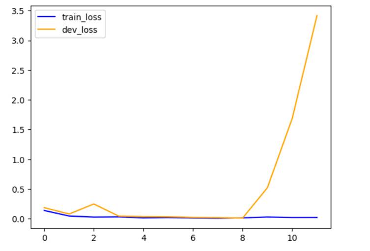
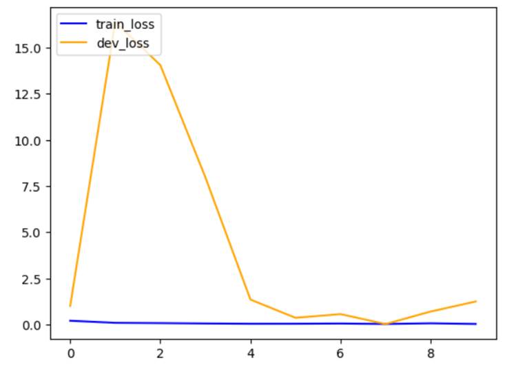
The train accuracy after the last epoch is 0.9760 and dev accuracy is 0.9245.
 
 

10. Now, I plotted a graph of train loss vs dev loss.

import matplotlib.pyplot as plt

plt.plot(history1.history['loss'],color='blue',label='train_loss')

plt.plot(history1.history['val_loss'],color='orange',label='dev_loss')

plt.legend(loc='upper left')

plt.show()

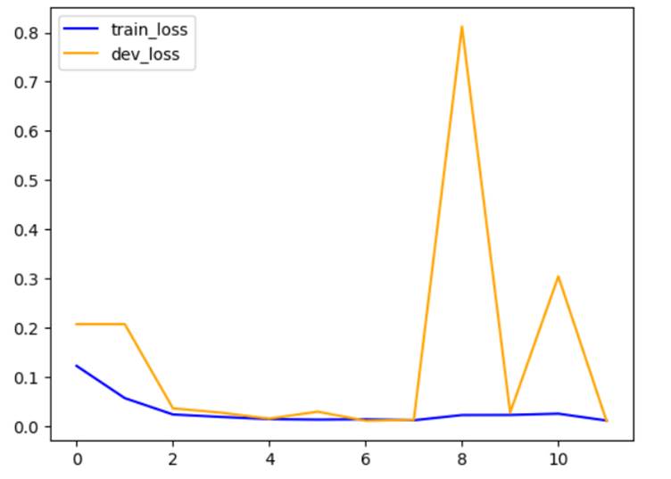
11. Now, I built another model by changing filters to 256 using 12 epochs.

from tensorflow.keras.applications import EfficientNetB2

backbone = EfficientNetB2(

input_shape=(96, 96, 3),

include_top=False

)

model2 = tf.keras.Sequential([

backbone,

tf.keras.layers.Conv2D(256, 3, padding='same', activation='relu'),

tf.keras.layers.GlobalAveragePooling2D(),

tf.keras.layers.Dense(256, activation='relu'),

tf.keras.layers.Dropout(0.3),

tf.keras.layers.Dense(8, activation='sigmoid')

])

model2.summary()

model2.compile(

optimizer=tf.keras.optimizers.Adam(learning_rate=0.001, beta_1=0.9, beta_2=0.999, epsilon=1e-07),

loss = 'binary_crossentropy',

metrics=['accuracy' , tf.keras.metrics.Precision(name='precision'),tf.keras.metrics.Recall(name='recall')]

)

history2 = model2.fit(

train_dataset,

steps_per_epoch=len(train_labels)//BATCH_SIZE,

epochs=12,

validation_data=val_dataset,

validation_steps = len(dev_labels)//BATCH_SIZE,

class_weight=class_weight

)

The train accuracy after the last epoch is 0.9910 and dev accuracy is 0.9870.
 

12. Now, I plotted a graph of train loss vs dev loss.

import matplotlib.pyplot as plt

plt.plot(history2.history['loss'],color='blue',label='train_loss')

plt.plot(history2.history['val_loss'],color='orange',label='dev_loss')

plt.legend(loc='upper left')

plt.show()

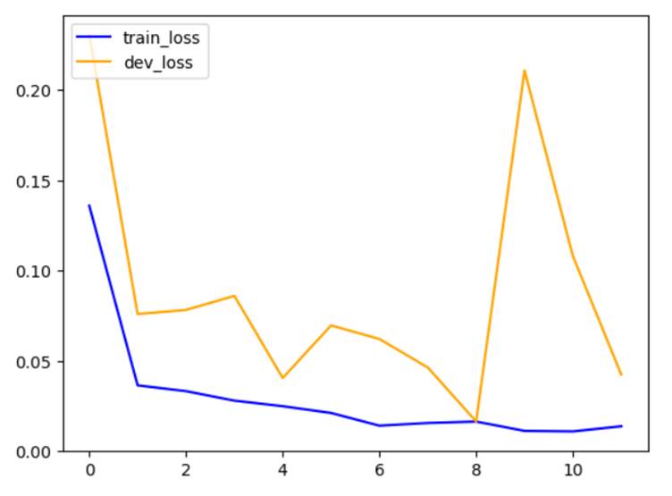
13. Now, I built another model using 256 filters and kernel size 4 using 12 epochs. Also, I used MaxPooling here.

from tensorflow.keras.applications import EfficientNetB2

backbone = EfficientNetB2(

input_shape=(96, 96, 3),

include_top=False

)

model3 = tf.keras.Sequential([

backbone,

tf.keras.layers.Conv2D(256, 4, padding='same', activation='relu'),

tf.keras.layers.MaxPooling2D((3,3)),

tf.keras.layers.Flatten(),

tf.keras.layers.Dense(256, activation='relu'),

tf.keras.layers.Dropout(0.3),

tf.keras.layers.Dense(8, activation='sigmoid')

])

model3.summary()

model3.compile(

optimizer=tf.keras.optimizers.Adam(learning_rate=0.001, beta_1=0.9, beta_2=0.999, epsilon=1e-07),

loss = 'binary_crossentropy',

metrics=['accuracy' , tf.keras.metrics.Precision(name='precision'),tf.keras.metrics.Recall(name='recall')])

history3 = model3.fit(

train_dataset,

steps_per_epoch=len(train_labels)//BATCH_SIZE,

epochs=12,

validation_data=val_dataset,

validation_steps = len(dev_labels)//BATCH_SIZE,

class_weight=class_weight

 The train accuracy after the last epoch is 0.9923 and dev accuracy is 0.9727.

14. Now, I plotted a graph of train loss vs dev loss.

import matplotlib.pyplot as plt

plt.plot(history3.history['loss'],color='blue',label='train_loss')

plt.plot(history3.history['val_loss'],color='orange',label='dev_loss')

plt.legend(loc='upper left')

plt.show()

15. Now, I built another model using 256 filters and kernel size 4 using 10 epochs. Also, I used MaxPooling here. Also changed learning rate from 0.001to 0.003 in optimizer.

from tensorflow.keras.applications import EfficientNetB2

backbone = EfficientNetB2(

input_shape=(96, 96, 3),

include_top=False

)

model4 = tf.keras.Sequential([

backbone,

tf.keras.layers.Conv2D(256, 4, padding='same', activation='relu'),

tf.keras.layers.MaxPooling2D((3,3), padding='same'),

tf.keras.layers.Conv2D(256, 4, padding='same', activation='relu'),

tf.keras.layers.MaxPooling2D((3,3), padding='same'),

tf.keras.layers.Flatten(),

tf.keras.layers.Dense(256, activation='relu'),

tf.keras.layers.Dropout(0.3),

tf.keras.layers.Dense(8, activation='sigmoid')

])

model4.summary()

model4.compile(

optimizer=tf.keras.optimizers.Adam(learning_rate=0.003, beta_1=0.9, beta_2=0.999, epsilon=1e-07),

loss = 'binary_crossentropy',

metrics=['accuracy' , tf.keras.metrics.Precision(name='precision'),tf.keras.metrics.Recall(name='recall')]

)

history4 = model4.fit(

train_dataset,

steps_per_epoch=len(train_labels)//BATCH_SIZE,

epochs=10,

validation_data=val_dataset,

validation_steps = len(dev_labels)//BATCH_SIZE,

class_weight=class_weight

)

The train accuracy after the last epoch is 0.9619 and dev accuracy is 0.6875. The dev accuracy has decreased a lot compared to the previous models.

16. Now, I plotted a graph of train loss vs dev loss.

import matplotlib.pyplot as plt

plt.plot(history4.history['loss'],color='blue',label='train_loss')

plt.plot(history4.history['val_loss'],color='orange',label='dev_loss')

plt.legend(loc='upper left')

plt.show()

17. In the above all models the dev accuracy is high in the second model. The hyperparameters are 256 filters, 3 kernels , average pooling and learning rate 0.001with 12 epochs.

from tensorflow.keras.applications import EfficientNetB2

backbone = EfficientNetB2(

input_shape=(96, 96, 3),

include_top=False

)

model_test = tf.keras.Sequential([

backbone,

tf.keras.layers.Conv2D(256, 3, padding='same', activation='relu'),

tf.keras.layers.GlobalAveragePooling2D(),

tf.keras.layers.Dense(256, activation='relu'),

tf.keras.layers.Dropout(0.3),

tf.keras.layers.Dense(8, activation='sigmoid')

])

model_test.summary()

model_test.compile(

optimizer=tf.keras.optimizers.Adam(learning_rate=0.001, beta_1=0.9, beta_2=0.999, epsilon=1e-07),

loss = 'binary_crossentropy',

metrics=['accuracy' , tf.keras.metrics.Precision(name='precision'),tf.keras.metrics.Recall(name='recall')]

)

history_test = model_test.fit(

train_dataset,

steps_per_epoch=len(train_labels)//BATCH_SIZE,

epochs=12,

validation_data=test_dataset,

validation_steps = len(dev_labels)//BATCH_SIZE,

class_weight=class_weight

)

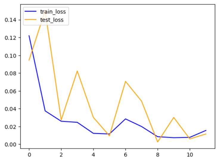
The train accuracy after the last epoch is 0.9863 and test accuracy is 0.9870.

18. Now, I plotted a graph of train loss vs test loss.

import matplotlib.pyplot as plt

plt.plot(history_test.history['loss'],color='blue',label='train_loss')

plt.plot(history_test.history['val_loss'],color='orange',label='test_loss')

plt.legend(loc='upper left')

plt.show()

K-nearest neighbors algorithm:

It is a supervised machine learning algorithm. It is simple and can be used for both regression and classification. The main idea in simple words is Tell me who your neighbors are, and I will tell you who you are. In order to classify one data point we will n neighbors of that data point. In that we will see the maximum members of the same class and assign that class to this data point. Here no training is required.

19. I used KNN algorithm on the entire dataset. First, I converted image path to pixels by adding a new column img_data. Then I resized the image and flattened to 1D array.

df['img_data'] = [cv2.imread(img_path) for img_path in df['img_path']]

from skimage.transform import resize

img_data_flat = np.array([resize(img, (100, 100)).flatten() for img in df['img_data']])

print(img_data_flat)

20. Now I applied KNN algorithm using 3 neighbors.

from sklearn.neighbors import KNeighborsClassifier

neigh = KNeighborsClassifier(n_neighbors=3)

neigh.fit(img_data_flat, df['class_names'])

accuracy = neigh.score(img_data_flat, df['class_names'])

print("Accuracy: ", accuracy)

 The accuracy is 0.8535

21. Similarly, I used various neighbors 5,7,9,11,13 and 15. The respective accuracies are

0.8535,0.78725,0.76425,0.73525,0.725,0.71025 and 0.7005. I plotted a graph.

x=[3,5,7,9,11,13,15]

y=[0.8535,0.78725,0.76425,0.73525,0.725,0.71025,0.7005]

plt.xlabel("Nieghbors")

plt.ylabel("Accurcay")

plt.plot(x,y)

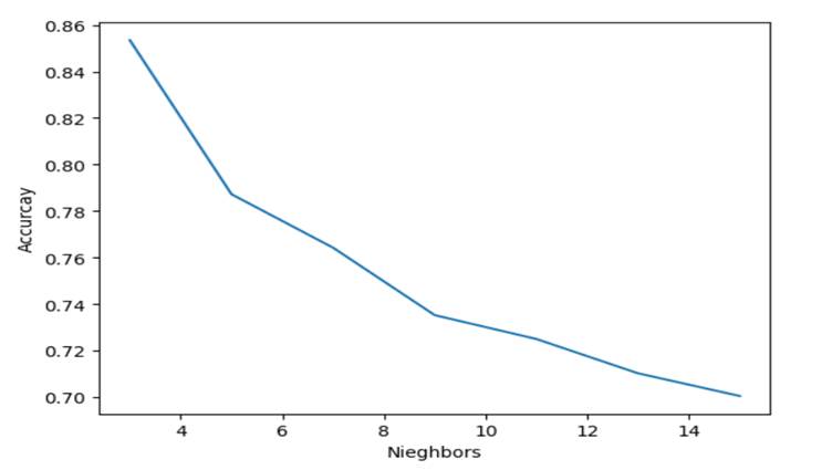
We can observe that as the number of neighbors increase, gradually the accuracy decreases.

Contribution:

1. I converted the data present in the directories to a data frame.

2. I performed label encoding and one hot encoding on the class names.

3. I built a CNN model and tried various models by changing filters, kernels and pooling layer.

4. I found the model which gives best accuracy on the dev dataset and applied that hyperparameters on the test dataset.

5. I also plotted graphs for train loss vs dev loss.

6. Next, I implemented KNN algorithm choosing various number of neighbors and plotted a graph for neighbors vs accuracy.

 Technical Challenges and solution:
1. Initially I faced difficulties while dealing with directories of data. Then I converted them a data frame which made my work easy.
2. Also, while using KNN algorithm, I faced difficulties while passing image data to the classifier. Then I resized and flattened the pixels array and continued the process.

References:

1] I watched explanation of CNN video in you tube. The link to the video is (7) Simple explanation of convolutional neural network | Deep Learning Tutorial 23 (Tensorflow & Python) - YouTube

2] In step 1 to convert directories to a data frame ,I used the code from this link. Facial expression | Kaggle

3] In step 2 to divide data into train, test, and dev, I used code from this link. How to split data into three sets (train, validation, and test) And why? | by Samarth Agrawal | Towards Data Science

4] In steps 3, 4, 5 , 6, 7 ,8,9 to perform all the required operations, I used the code from this link. Facial expression | Kaggle

5] In step 10 to plot a graph , I referred you tube video to plot graphs. The link is (7) Build a Deep CNN Image Classifier with ANY Images - YouTube

6] To explain KNN algorithm, I referred the following links. Machine Learning Basics with the K-Nearest Neighbors Algorithm | by Onel Harrison | Towards Data Science and k-NN classifier for image classification PyIm ageSearch

7] In steps 19, 20 to implement KNN algorithm, I used the code from this link. k-NN classifier for image classification - PyImageSearch

Source Code
Github link
Kaggle link
Youtube video